Computing Your Skill
Summary: I describe how the TrueSkill algorithm works using concepts you’re already familiar with. TrueSkill is used on Xbox Live to rank and match players and it serves as a great way to understand how statistical machine learning is actually applied today. I’ve also created an open source project where I implemented TrueSkill three different times in increasing complexity and capability. In addition, I’ve created a detailed supplemental math paper that works out equations that I gloss over here. Feel free to jump to sections that look interesting and ignore ones that seem boring. Don’t worry if this post seems a bit long, there are lots of pictures.
Introduction
It seemed easy enough: I wanted to create a database to track the skill levels of my coworkers in chess and foosball. I already knew that I wasn’t very good at foosball and would bring down better players. I was curious if an algorithm could do a better job at creating well-balanced matches. I also wanted to see if I was improving at chess. I knew I needed to have an easy way to collect results from everyone and then use an algorithm that would keep getting better with more data. I was looking for a way to compress all that data and distill it down to some simple knowledge of how skilled people are. Based on some previous things that I had heard about, this seemed like a good fit for “machine learning.”
But, there’s a problem.
Machine learning is a hot area in Computer Science— but it’s intimidating. Like most subjects, there’s a lot to learn to be an expert in the field. I didn’t need to go very deep; I just needed to understand enough to solve my problem. I found a link to the paper describing the TrueSkill algorithm and I read it several times, but it didn’t make sense. It was only 8 pages long, but it seemed beyond my capability to understand. I felt dumb. Even so, I was too stubborn to give up. Jamie Zawinski said it well:
“Not knowing something doesn’t mean you’re dumb— it just means you don’t know it.”
I learned that the problem isn’t the difficulty of the ideas themselves, but rather that the ideas make too big of a jump from the math that we typically learn in school. This is sad because underneath the apparent complexity lies some beautiful concepts. In hindsight, the algorithm seems relatively simple, but it took me several months to arrive at that conclusion. My hope is that I can short-circuit the haphazard and slow process I went through and take you directly to the beauty of understanding what’s inside the gem that is the TrueSkill algorithm.
Skill ≈ Probability of Winning

Skill is tricky to measure. Being good at something takes deliberate practice and sometimes a bit of luck. How do you measure that in a person? You could just ask someone if they’re skilled, but this would only give a rough approximation since people tend to be overconfident in their ability. Perhaps a better question is “what would the units of skill be?” For something like the 100 meter dash, you could just average the number of seconds of several recent sprints. However, for a game like chess, it’s harder because all that’s really important is if you win, lose, or draw.
It might make sense to just tally the total number of wins and losses, but this wouldn’t be fair to people that played a lot (or a little). Slightly better is to record the percent of games that you win. However, this wouldn’t be fair to people that beat up on far worse players or players who got decimated but maybe learned a thing or two. The goal of most games is to win, but if you win too much, then you’re probably not challenging yourself. Ideally, if all players won about half of their games, we’d say things are balanced. In this ideal scenario, everyone would have a near 50% win ratio, making it impossible to compare using that metric.
Finding universal units of skill is too hard, so we’ll just give up and not use any units. The only thing we really care about is roughly who’s better than whom and by how much. One way of doing this is coming up with a scale where each person has a unit-less number expressing their rating that you could use for comparison. If a player has a skill rating much higher than someone else, we’d expect them to win if they played each other.
The key idea is that a single skill number is meaningless. What’s important is how that number compares with others. This is an important point worth repeating: skill only makes sense if it’s relative to something else. We’d like to come up with a system that gives us numbers that are useful for comparing a person’s skill. In particular, we’d like to have a skill rating system that we could use to predict the probability of winning, losing, or drawing in matches based on a numerical rating.
We’ll spend the rest of our time coming up with a system to calculate and update these skill numbers with the assumption that they can be used to determine the probability of an outcome.
What Exactly is Probability Anyway?
You can learn about probability if you’re willing to flip a coin— a lot. You flip a few times:


Heads, heads, tails!
Each flip has a seemingly random outcome. However, “random” usually means that you haven’t looked long enough to see a pattern emerge. If we take the total number of heads and divide it by the total number of flips, we see a very definite pattern emerge:
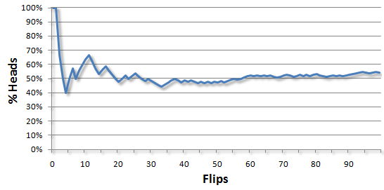
But you knew that it was going to be a 50-50 chance in the long run. When saying something is random, we often mean it’s bounded within some range. 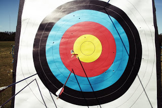
It turns out that a better metaphor is to think of a bullseye that archers shoot at. Each arrow will land somewhere near that center. It would be extraordinary to see an arrow hit the bullseye exactly. Most of the arrows will seem to be randomly scattered around it. Although “random,” it’s far more likely that arrows will be near the target than, for example, way out in the woods (well, except if I was the archer).
This isn’t a new metaphor; the Greek word στόχος (stochos) refers to a stick set up to aim at. It’s where statisticians get the word stochastic: a fancy, but slightly more correct word than random. The distribution of arrows brings up another key point:
All things are possible, but not all things are probable.
Probability has changed how ordinary people think, a feat that rarely happens in mathematics. The very idea that you could understand anything about future outcomes is such a big leap in thought that it baffled Blaise Pascal, one of the best mathematicians in history.
In the summer of 1654, Pascal exchanged a series of letters with Pierre de Fermat, another brilliant mathematician, concerning an “unfinished game.” Pascal wanted to know how to divide money among gamblers if they have to leave before the game is finished. Splitting the money fairly required some notion of the probability of outcomes if the game would have been played until the end. This problem gave birth to the field of probability and laid the foundation for lots of fun things like life insurance, casino games, and scary financial derivatives.
But probability is more general than predicting the future— it’s a measure of your ignorance of something. It doesn’t matter if the event is set to happen in the future or if it happened months ago. All that matters is that you lack knowledge in something. Just because we lack knowledge doesn’t mean we can’t do anything useful, but we’ll have to do a lot more coin flips to see it.
Aggregating Observations
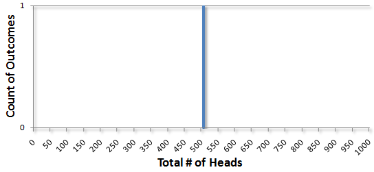
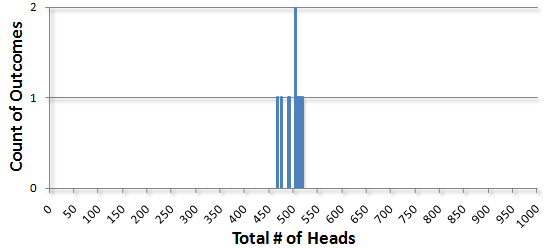
The real magic happens when we aggregate a lot of observations. What would happen if you flipped a coin 1000 times and counted the number of heads? Lots of things are possible, but in my case I got 505 heads. That’s about half, so it’s not surprising. I can graph this by creating a bar chart and put all the possible outcomes (getting 0 to 1000 heads) on the bottom and the total number of times that I got that particular count of heads on the vertical axis. For 1 outcome of 505 total heads it would look like this:
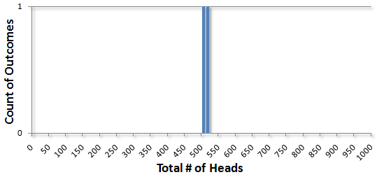
Not too exciting. But what if we did it again? This time I got 518 heads. I can add that to the chart:
Doing it 8 more times gave me 489, 515, 468, 508, 492, 475, 511, and once again, I got 505. The chart now looks like this:
And after a billion times, a total of one trillion flips, I got this:

In all the flips, I never got less than 407 total heads and I never got more than 600. Just for fun, we can zoom in on this region:
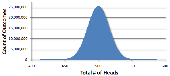
As we do more sets of flips, the jagged edges smooth out to give us the famous “bell curve” that you’ve probably seen before. Math guys love to refer to it as a “Gaussian” curve because it was used by the German mathematician Carl Gauss in 1809 to investigate errors in astronomical data. He came up with an exact formula of what to expect if we flipped a coin an infinite number of times (so that we don’t have to). This is such a famous result that you can see the curve and its equation if you look closely at the middle of an old 10 Deutsche Mark banknote bearing Gauss’s face:
 USA currency?")
Don’t miss the forest from all the flippin’ trees. The curve is showing you the density of all possible outcomes. By density, I mean how tall the curve gets at a certain point. For example, in counting the total number of heads out of 1000 flips, I expected that 500 total heads would be the most popular outcome and indeed it was. I saw 25,224,637 out of a billion sets that had exactly 500 heads. This works out to about 2.52% of all outcomes. In contrast, if we look at the bucket for 450 total heads, I only saw this happen 168,941 times, or roughly 0.016% of the time. This confirms your observation that the curve is denser, that is, taller at the mean of 500 than further away at 450.
This confirms the key point: all things are possible, but outcomes are not all equally probable. There are longshots. Professional athletes panic or ‘choke’. The world’s best chess players have bad days. Additionally, tales about underdogs make us smile— the longer the odds the better. Unexpected outcomes happen, but there’s still a lot of predictability out there.
It’s not just coin flips. The bell curve shows up in lots of places like casino games, to the thickness of tree bark, to the measurements of a person’s IQ. Lots of people have looked at the world and have come up with Gaussian models. It’s easy to think of the world as one big, bell shaped playground.
But the real world isn’t always Gaussian. History books are full of “Black Swan” events. Stock market crashes and the invention of the computer are statistical outliers that Gaussian models tend not to predict well, but these events shock the world and forever change it. This type of reality isn’t covered by the bell curve, what Black Swan author Nassim Teleb calls the “Great Intellectual Fraud.” These events would have such low probability that no one would predict them actually happening. There’s a different view of randomness that is a fascinating playground of Benoît Mandelbrot and his fractals that better explain some of these events, but we will ignore all of this to keep things simple. We’ll acknowledge that the Gaussian view of the world isn’t always right, no more than a map of the world is the actual terrain.
The Gaussian worldview assumes everything will typically be some average value and then treats everything else as increasingly less likely “errors” as you exponentially drift away from the center (Gauss used the curve to measure errors in astronomical data after all). However, it’s not fair to treat real observations from the world as “errors” any more than it is to say that a person is an “error” from the “average human” that is half male and half female. Some of these same problems can come up treating a person as having skill that is Gaussian. Disclaimers aside, we’ll go along with George Box’s view that “all models are wrong, but some models are useful.”
Gaussian Basics
Gaussian curves are completely described by two values:
- The mean (average) value which is often represented by the Greek letter μ (mu)
- The standard deviation, represented by the Greek letter σ (sigma). This indicates how far apart the data is spread out.
In counting the total number heads in 1000 flips, the mean was 500 and the standard deviation was about 16. In general, 68% of the outcomes will be within ± 1 standard deviation (e.g. 484-516 in the experiment), 95% within 2 standard deviations (e.g. 468-532) and 99.7% within 3 standard deviations (452-548):
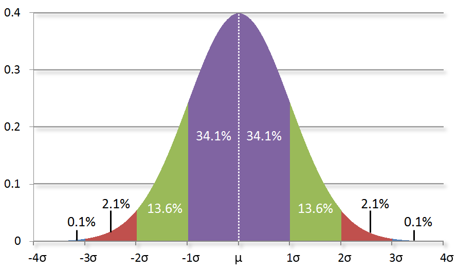
An important takeaway is that the bell curve allows for all possibilities, but each possibility is most definitely not equally likely. The bell curve gives us a model to calculate how likely something should be given an average value and a spread. Notice how outcomes sharply become less probable as we drift further away from the mean value.
While we’re looking at the Gaussian curve, it’s important to look at -3σ away from the mean on the left side. As you can see, most of the area under the curve is to the right of this point. I mention this because the TrueSkill algorithm uses the -3σ mark as a (very) conservative estimate for your skill. You’re probably better than this conservative estimate, but you’re most likely not worse than this value. Therefore, it’s a stable number for comparing yourself to others and is useful for use in sorting a leaderboard.
3D Bell Curves: Multivariate Gaussians
A non-intuitive observation is that Gaussian distributions can occur in more than the two dimensions that we’ve seen so far. You can sort of think of a Gaussian in three dimensions as a mountain. Here’s an example:

In this plot, taller regions represent higher probabilities. As you can see, not all things are equally probable. The most probable value is the mean value that is right in the middle and then things sharply decline away from it.
In maps of real mountains, you often see a 2D contour plot where each line represents a different elevation (e.g. every 100 feet):

The closer the lines on the map, the sharper the inclines. You can do something similar for 2D representations of 3D Gaussians. In textbooks, you often just see 2D representation that looks like this:

This is called an “isoprobability contour” plot. It’s just a fancy way of saying “things that have the same probability will be the same color.” Note that it’s still in three dimensions. In this case, the third dimension is color intensity instead of the height you saw on a surface plot earlier. I like to think of contour plots as treasure maps for playing the “you’re getting warmer…” game. In this case, black means “you’re cold,” red means “you’re getting warmer…,” and yellow means “you’re on fire!” which corresponds to the highest probability.
See? Now you understand Gaussians and know that “multivariate Gaussians” aren’t as scary as they sound.
Let’s Talk About Chess

There’s still more to learn, but we’ll pick up what we need along the way. We already have enough tools to do something useful. To warm up, let’s talk about chess because ratings are well-defined there.
In chess, a bright beginner is expected to have a rating around 1000. Keep in mind that ratings have no units; it’s just a number that is only meaningful when compared to someone else’s number. By tradition, a difference of 200 indicates the better ranked player is expected to win 75% of the time. Again, nothing is special about the number 200, it was just chosen to be the difference needed to get a 75% win ratio and effectively defines a “class” of player.
I’ve slowly been practicing and have a rating around 1200. This means that if I play a bright beginner with a rating of 1000, I’m expected to win three out of four games.
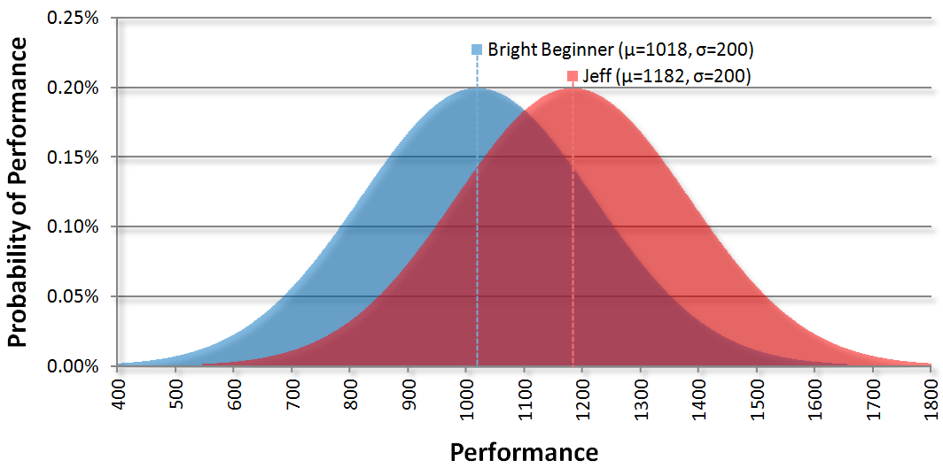
We can start to visualize a match between me and bright beginner by drawing two bell curves that have a mean of 1000 and 1200 respectively with both having a standard deviation of 200:
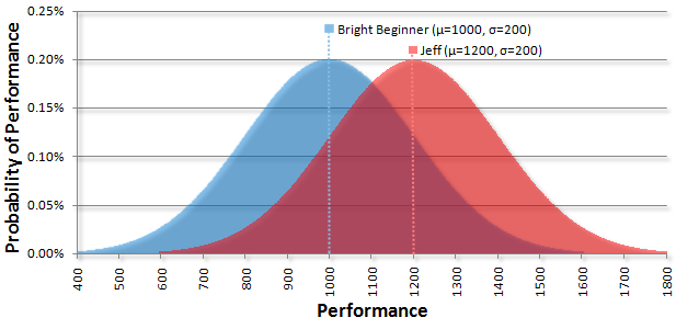
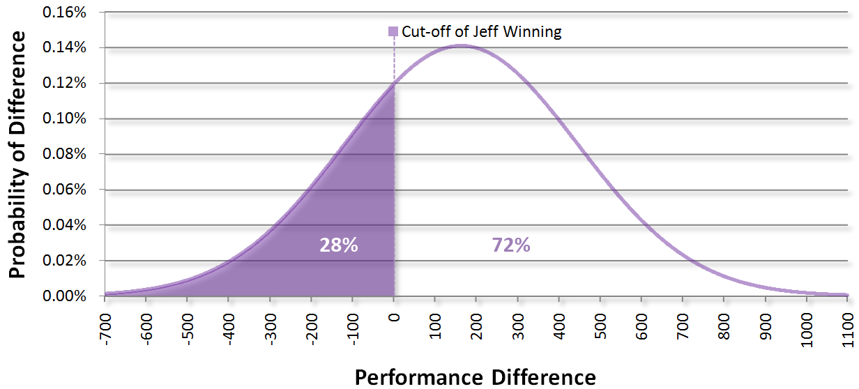
The above graph shows what the ratings represent: they’re an indicator of how we’re expected to perform if we play a game. The most likely performance is exactly what the rating is (the mean value). One non-obvious point is that you can subtract two bell curves and get another bell curve. The new center is the difference of the means and the resulting curve is a bit wider than the previous curves. By taking my skill curve (red) and subtracting the beginner’s curve (blue), you’ll get this resulting curve (purple):
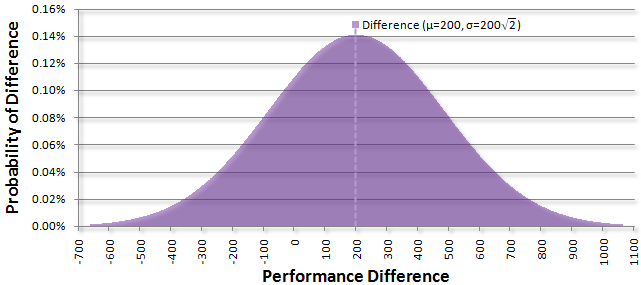
Note that it’s centered at 1200 - 1000 = 200. Although interesting to look on its own, it gives some useful information. This curve is representing all possible game outcomes between me and the beginner. The middle shows that I’m expected to be 200 points better. The far left side shows that there is a tiny chance that the beginner has a game where he plays as if he’s 700 points better than I am. The far right shows that there is a tiny chance that I’ll play as if I’m 1100 points better. The curve actually goes on forever in both ways, but the expected probability for those outcomes is so small that it’s effectively zero.
As a player, you really only care about one very specific point on this curve: zero. Since I have a higher rating, I’m interested in all possible outcomes where the difference is positive. These are the outcomes where I’m expected to outperform the beginner. On the other hand, the beginner is keeping his eye on everything to the left of zero. These are the outcomes where the performance difference is negative, implying that he outperforms me.
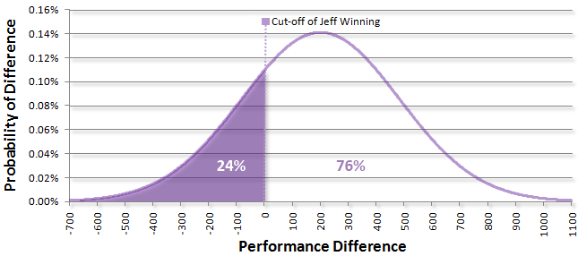
We can plug a few numbers into a calculator and see that there is about a 24% probability that the performance difference will be negative, implying the beginner wins, and a 76% chance that the difference will be positive, meaning that I win. This is roughly the 75% that we were expecting for a 200 point difference.
This has been a bit too concrete for my particular match with a beginner. We can generalize it by creating another curve where the horizontal axis represents the difference in player ratings and the vertical axis represents the total probability of winning given that rating difference:
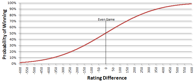
As expected, having two players with equal ratings, and thus a rating difference of 0, implies the odds of winning are 50%. Likewise, if you look at the -200 mark, you see the curve is at the 24% that we calculated earlier. Similarly, +200 is at the 76% mark. This also shows that outcomes on the far left side are quite unlikely. For example, the odds of me winning a game against Magnus Carlsen, who is at the top of the chess leaderboard with a rating of 2813, would be at the -1613 mark (1200 - 2813) on this chart and have a probability near one in a billion. I won’t hold my breath. (Actually, most chess groups use a slightly different curve, but the ideas are the same. See the accompanying math paper for details.)
All of these curves were probabilities of what might happen, not what actually happened. In actuality, let’s say I lost the game by some silly blunder (oops!). The question that the beginner wants to know is how much his rating will go up. It also makes sense that my rating will go down as a punishment for the loss. The harder question is just how much should the ratings change?
By winning, the beginner demonstrated that he was probably better than the 25% winning probability we thought he would have. One way of updating ratings is to imagine that each player bets a certain amount of his rating on each game. The amount of the bet is determined by the probability of the outcome. In addition, we decide how dramatic the ratings change should be for an individual game. If you believe the most recent game should count 100%, then you’d expect my rating to go down a lot and his to go up a lot. The decision of how much the most recent game should count leads to what chess guys call the multiplicative “K-factor.”
The K-Factor is what we multiply a probability by to get the total amount of a rating change. It reflects the maximum possible change in a person’s rating. A reasonable choice of a weight is that the most recent game counts about 7% which leads to a K-factor of 24. New players tend to have more fluctuations than well-established players, so new players might get a K-Factor of 32 while grand masters have a K-factor around
10. Here’s how the K-Factor changes with respect to how much the latest game should count:
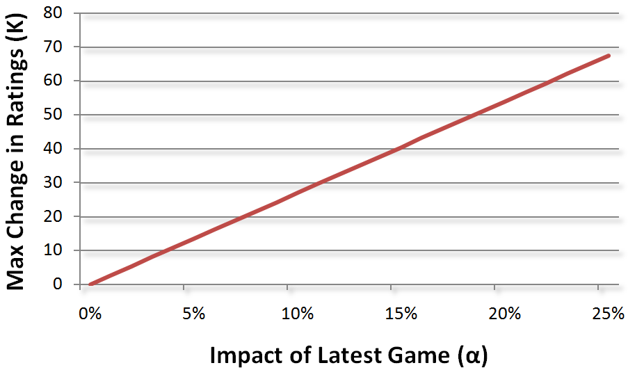
Using a K-Factor of 24 means that my rating will now be lowered to 1182 and the beginner’s will rise to 1018. Our curves are now closer together:
Note that our standard deviations never change. Here are the probabilities if we were to play again:
This method is known as the Elo rating system, named after Arpad Elo, the chess enthusiast who created it. It’s relatively simple to implement and most games that calculate skill end here.
I Thought You Said You’d Talk About TrueSkill?
Everything so far has just been prerequisites to the main event; the TrueSkill paper assumes you’re already familiar with it. It was all sort of new to me, so it took awhile to get comfortable with the Elo ideas. Although the Elo model will get you far, there are a few notable things it doesn’t handle well:
- Newbies - In the Elo system, you’re typically assigned a “provisional” rating for the first 20 games. These games tend to have a higher K-factor associated with them in order to let the algorithm determine your skill faster before it’s slowed down by a non-provisional (and smaller) K-factor. We would like an algorithm that converges quickly onto a player’s true skill (get it?) to not waste their time having unbalanced matches. This means the algorithm should start giving reasonable approximations of skill within 5-10 games.
- Teams - Elo was explicitly designed for two players. Efforts to adapt it to work for multiple people on multiple teams have primarily been unsophisticated hacks. One such approach is to treat teams as individual players that duel against the other players on the opposing teams and then apply the average of the duels. This is the “duelling heuristic” mentioned in the TrueSkill paper. I implemented it in the accompanying project. It’s ok, but seems a bit too hackish and doesn’t converge well.
- Draws - Elo treats draws as a half win and half loss. This doesn’t seem fair because draws can tell you a lot. Draws imply you were evenly paired whereas a win indicates you’re better, but unsure how much better. Likewise, a loss indicates you did worse, but you don’t really know how much worse. So it seems that a draw is important to explicitly model.
The TrueSkill algorithm generalizes Elo by keeping track of two variables: your average (mean) skill and the system’s uncertainty about that estimate (your standard deviation). It does this instead of relying on a something like a fixed K-factor. Essentially, this gives the algorithm a dynamic k-factor. This addresses the newbie problem because it removes the need to have “provisional” games. In addition, it addresses the other problems in a nice statistical manner. Tracking these two values are so fundamental to the algorithm that Microsoft researchers informally referred to it as the μσ (mu-sigma) system until the marketing guys gave it the name TrueSkill.
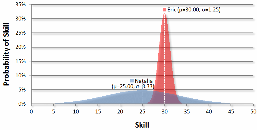
We’ll go into the details shortly, but it’s helpful to get a quick visual overview of what TrueSkill does. Let’s say we have Eric, an experienced player that has played a lot and established his rating over time. In addition, we have newbie: Natalia.
Here’s what their skill curves might look like before a game:
And after Natalia wins:
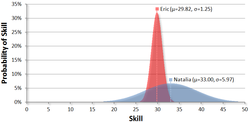
Notice how Natalia’s skill curve becomes narrower and taller (i.e. makes a big update) while Eric’s curve barely moves. This shows that the TrueSkill algorithm thinks that she’s probably better than Eric, but doesn’t how much better. Although TrueSkill is a little more confident about Natalia’s mean after the game (i.e. it’s now taller in the middle), it’s still very uncertain. Looking at her updated bell curve shows that her skill could be between 15 and 50.
The rest of this post will explain how calculations like this occurred and how much more complicated scenarios can occur. But to understand it well enough to implement it, we’ll need to learn a couple of new things.
Bayesian Probability
Most basic statistics classes focus on frequencies of events occurring. For example, the probability of getting a red marble when randomly drawing from a jar that has 3 red marbles and 7 blue marbles is 30%. Another example is that the probability of rolling two dice and getting a total of 7 is about 17%. The key idea in both of these examples is that you can count each type of outcome and then compute the frequency directly. Although helpful in calculating your odds at casino games, “frequentist” thinking is not that helpful with many practical applications, like finding your skill in a team.
A different approach is to think of probability as degree of belief in something. The basic idea is that you have some prior belief and then you observe some evidence that updates your belief leaving you with an updated posterior belief. As you might expect, learning about new evidence will typically make you more certain about your belief.
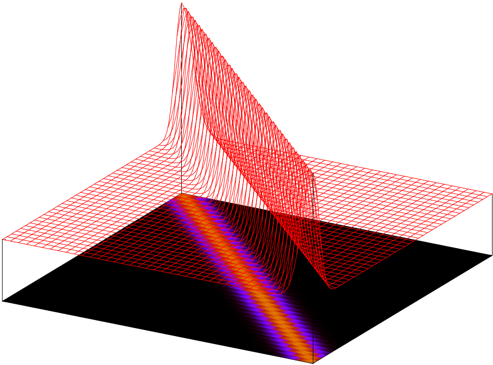
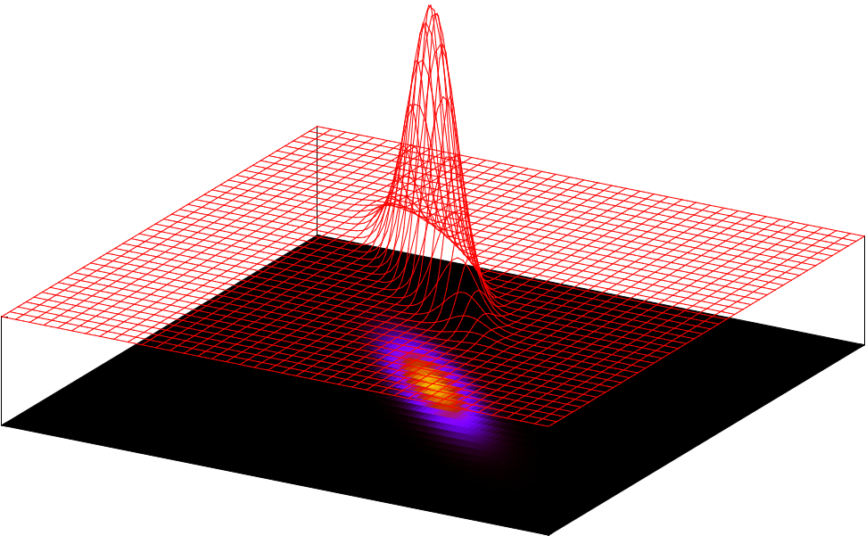
Let’s assume that you’re trying to find a treasure on a map. The treasure could be anywhere on the map, but you have a hunch that it’s probably around the center of the map and increasingly less likely as you move away from the center. We could track the probability of finding the treasure using the 3D multivariate Gaussian we saw earlier:
Now, let’s say that after studying a book about the treasure, you’ve learned that there’s a strong likelihood that treasure is somewhere along the diagonal line on the map. Perhaps this was based on some secret clue. Your clue information doesn’t necessarily mean the treasure will be exactly on that line, but rather that the treasure will most-likely be near it. The likelihood function might look like this in 3D:
We’d like to use our prior information and this new likelihood information to come up with a better posterior guess of the treasure. It turns out that we can just multiply the prior and likelihood to obtain a posterior distribution that looks like this:
This is giving us a smaller and more concentrated area to look at.
If you look at most textbooks, you typically just see this information using 2D isoprobability contour plots that we learned about earlier. Here’s the same information in 2D:
Prior:

Likelihood:

Posterior:

For fun, let’s say we found additional information saying the treasure is along the other diagonal with the following likelihood:

To incorporate this information, we’re able to take our last posterior and make that the prior for the next iteration using the new likelihood information to get this updated posterior:

This is a much more focused estimate than our original belief! We could iterate the procedure and potentially get an even smaller search area.
 And that’s basically all there is to it. In TrueSkill, the buried treasure that we look for is a person’s skill. This approach to probability is called “Bayesian” because it was discovered by a Presbyterian minister in the 1700’s named Thomas Bayes who liked to dabble in math.
The central ideas to Bayesian statistics are the prior, the likelihood, and the posterior. There’s detailed math that goes along with this and is in the accompanying paper, but understanding these basic ideas is more important:
“When you understand something, then you can find the math to express that understanding. The math doesn’t provide the understanding.”— Lamport
Bayesian methods have only recently become popular in the computer age because computers can quickly iterate through several tedious rounds of priors and posteriors. Bayesian methods have historically been popular inside of Microsoft Research (where TrueSkill was invented). Way back in 1996, Bill Gates considered Bayesian statistics to be Microsoft Research’s secret sauce.
As we’ll see later on, we can use the Bayesian approach to calculate a person’s skill. In general, it’s highly useful to update your belief based off previous evidence (e.g. your performance in previous games). This usually works out well. However, sometimes “Black Swans” are present. For example, a turkey using Bayesian inference would have a very specific posterior distribution of the kindness of a farmer who feeds it every day for 1000 days only to be surprised by a Thanksgiving event that was so many standard deviations away from the turkey’s mean belief that he never would have saw it coming. Skill has similar potential for a “Thanksgiving” event where an average player beats the best player in the world. We’ll acknowledge that small possibility, but ignore it to simplify things (and give the unlikely winner a great story for the rest of his life).
TrueSkill claims that it is Bayesian, so you can be sure that there is going to be a concept of a prior and a likelihood in it— and there is. We’re getting closer, but we still need to learn a few more details.
The Marginalized, but Not Forgotten Distribution
 Next we need to learn about “marginal distributions”, often just called “marginals.” Marginals are a way of distilling information to focus on what you care about. Imagine you have a table of sales for each month for the past year. Let’s say that you only care about total sales for the year. You could take out your calculator and add up all the sales in each month to get the total aggregate sales for the year. Since you care about this number and it wasn’t in the original report, you could add it in the margin of the table. That’s roughly where “margin-al” got its name.
Wikipedia has a great illustration on the topic: consider a guy that ignores his mom’s advice and never looks both ways when crossing the street. Even worse, he’s too engrossed in listening to his iPod that he doesn’t look any way, he just always crosses.
What’s the probability of him getting hit by a car at a specific intersection? Let’s simplify things by saying that it just depends on whether the light is red, yellow, or green.
| Light State | Red | Yellow | Green |
|---|---|---|---|
| Probability of getting hit given light state | 1% | 9% | 90% |
This is helpful, but it doesn’t tell us what we want. We also need to know how long the light stays a given color
| Light color | Red | Yellow | Green |
|---|---|---|---|
| % Time in Color | 60% | 10% | 30% |
There’s a bunch of probability data here that’s a bit overwhelming. If we join the probabilities together, we’ll have a “joint distribution” that’s just a big complicated system that tells us too much information.
We can start to distill this information down by calculating the probability of getting hit given each light state:
| Red | Yellow | Green | Total Probability of Getting Hit |
|---|---|---|---|
| 1%*60% = 0.6% | 9%*10% = 0.9% | 90%*30% = 27% | 28.5% |
In the right margin of the table we get the value that really matters to this guy. There’s a 28.5% marginal probability of getting hit if the guy never looks for cars and just always crosses the street. We obtained it by “summing out” the individual components. That is, we simplified the problem by eliminating variables and we eliminated variables by just focusing on the total rather than the parts.
This idea of marginalization is very general. The central question in this article is “computing your skill,” but your skill is complicated. When using Bayesian statistics, we often can’t observe something directly, so we have to come up with a probability distribution that’s more complicated and then “marginalize” it to get the distribution that we really want. We’ll need to marginalize your skill by doing a similar “summing-out” procedure as we did for the reckless guy above.
But before we do that, we need to learn another technique to make calculations simpler.
What’s a Factor Graph, and Why Do I Care?
Remember your algebra class when you worked with expressions like this?
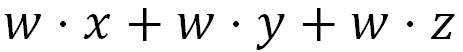
Your teacher showed you that you could simplify this by “factor-ing” out w, like this:
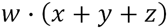
We often factor expressions to make them easier to understand and to simplify calculations. Let’s replace the variables above with w=4, x=1, y=2, and z=3.
Let’s say the numbers on our calculator are circles and the operators are squares. We could come up with an “expression tree” to describe the calculation like this:
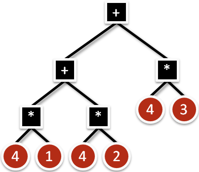
You can tell how tedious this computation is by counting 11 “buttons” we’d have to push. We could also factor it like this
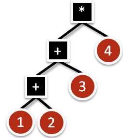
This “factorization” has a total of 7 buttons, a savings of 4 buttons. It might not seem like much here, but factorizing is a big idea.
We face a similar problem of how to factor things when we’re looking to simplify a complicated probability distribution. We’ll soon see how your skill is composed of several “factors” in a joint distribution. We can simplify computations based on how variables are related to these factors. We’ll break up the joint distribution into a bunch of factors on a graph. This graph that links factors and variables is called a “factor graph.”
The key idea about a factor graph is that we represent the marginal conditional probabilities as variables and then represent each major function of those variables as a “factor.” We’ll take advantage of how the graph “factorizes” and imagine that each factor is a node on a network that’s optimized for efficiency. A key efficiency trick is that factor nodes send “messages” to other nodes. These messages help simplify further marginal computations. The “message passing” is very important and thus will be highlighted with arrows in the upcoming graphs; gray arrows represent messages going “down” the graph and black show messages coming “up” the graph.
The accompanying code and math paper go into details about exactly how this happens, but it’s important to realize the high level idea first. That is, we want to look at all the factors that go into creating the likelihood function for updating a person’s skill based on a game outcome. Representing this information in a factor graph helps us see how things are related.
Now we have all the foundational concepts that we’re ready for the main event: the TrueSkill factor graph!
Enough Chess, Let’s Rank Something Harder!
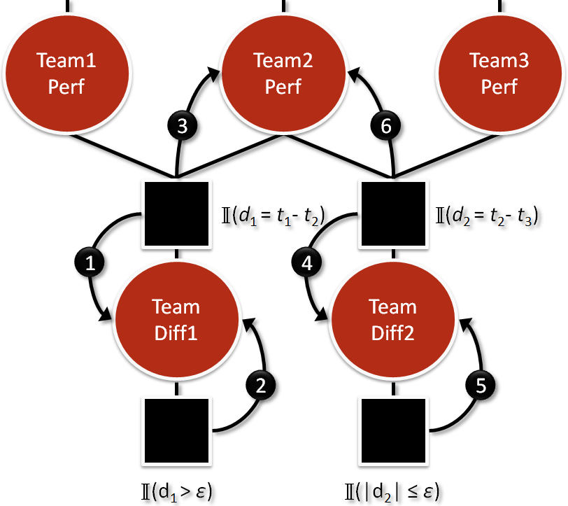
The TrueSkill algorithm is Bayesian because it’s composed of a prior multiplied by a likelihood. I’ve highlighted these two components in the sample factor graph from the TrueSkill paper that looks scary at first glance:
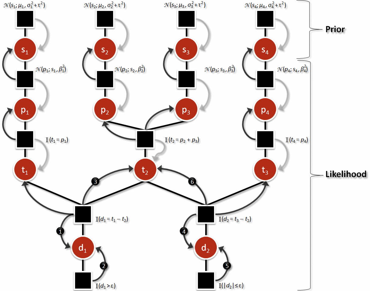
This factor graph shows the outcome of a match that had 3 teams all playing against each other. The first team (on the left) only has one player, but this player was able to defeat both of the other teams. The second team (in the middle) had two players and this team tied the third team (on the right) that had just one player.
In TrueSkill, we just care about a player’s marginal skill. However, as is often the case with Bayesian models, we have to explicitly model other things that impact the variable we care about. We’ll briefly cover each factor (more details are in the code and math paper).
Factor #1: What Do We Already Know About Your Skill?
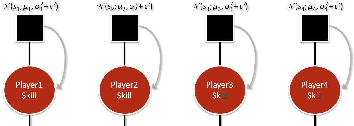
The first factor starts the whole process. It’s where we get a player’s previous skill level from somewhere (e.g. a player database). At this point, we add some uncertainty to your skill’s standard deviation to keep game dynamics interesting and prevent the standard deviation from hitting zero since the rest of algorithm will make it smaller (since the whole point is to learn about you and become more certain).
There is a factor and a variable for each player. Each factor is a function that remembers a player’s previous skill. Each variable node holds the current value of a player’s skill. I say “current” because this is the value that we’ll want to know about after the whole algorithm is completed. Note that the message arrow on the factor only goes one way; we never go back to the prior factor. It just gets things going. However, we will come back to the variable.
But we’re getting ahead of ourselves.
Factor #2: How Are You Going To Perform?
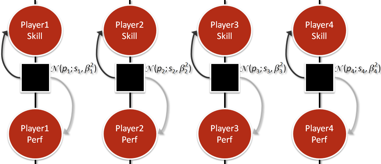
Next, we add in beta (β). You can think of beta as the number of skill points to guarantee about an 80% chance of winning. The TrueSkill inventors refer to beta as defining the length of a “skill chain.”
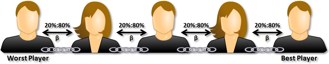
The skill chain is composed of the worst player on the far left and the best player on the far right. Each subsequent person on the skill chain is “beta” points better and has an 80% win probability against the weaker player. This means that a small beta value indicates a high-skill game (e.g. Go) since smaller differences in points lead to the 80%:20% ratio. Likewise, a game based on chance (e.g. Uno) is a low-skill game that would have a higher beta and smaller skill chain.
Factor #3: How is Your Team Going to Perform?
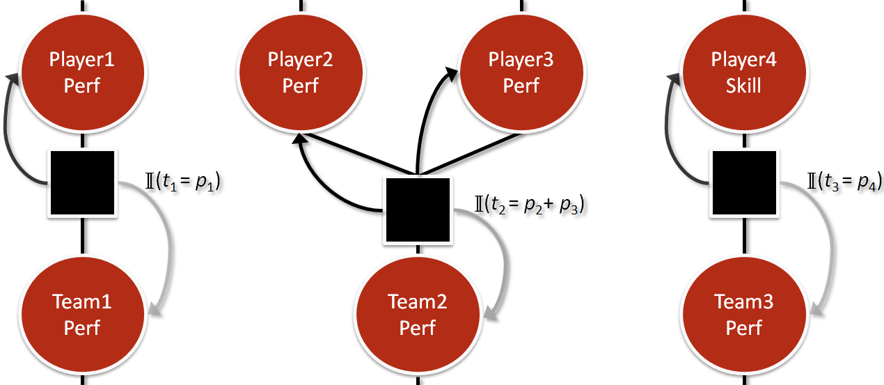
Now we’re ready for one of the most controversial aspects of TrueSkill: computing the performance of a team as a whole. In TrueSkill, we assume the team’s performance is the sum of each team member’s performance. I say that it’s “controversial” because some members of the team probably work harder than others. Additionally, sometimes special dynamics occur that make the sum greater than the parts. However, we’ll fight the urge to make it much more complicated and heed Makridakis’s advice:
“Statistically sophisticated or complex methods do not necessarily provide more accurate forecasts than simpler ones”
One cool thing about this factor is that you can weight each team member’s contribution by the amount of time that they played. For example, if two players are on a team but each player only played half of the time (e.g. a tag team), then we would treat them differently than if these two players played the entire time. This is officially known as “partial play.” Xbox game titles report the percentage of time a player was active in a game under the “X_PROPERTY_PLAYER_PARTIAL_PLAY_PERCENTAGE” property that is recorded for each player (it defaults to 100%). This information is used by TrueSkill to perform a fairer update. I implemented this feature in the accompanying source code.
Factor #4: How’d Your Team Compare?
Next, we compare team performances in pairs. We do this by subtracting team performances to come up with pairwise differences:
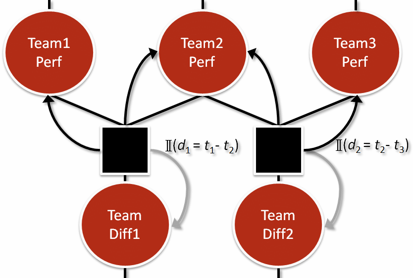
This is similar to what we did earlier with Elo and subtracting curves to get a new curve.
Factor #5: How Should We Interpret the Team Differences?
The bottom of the factor graph contains a comparison factor based on the team performance differences we just calculated:
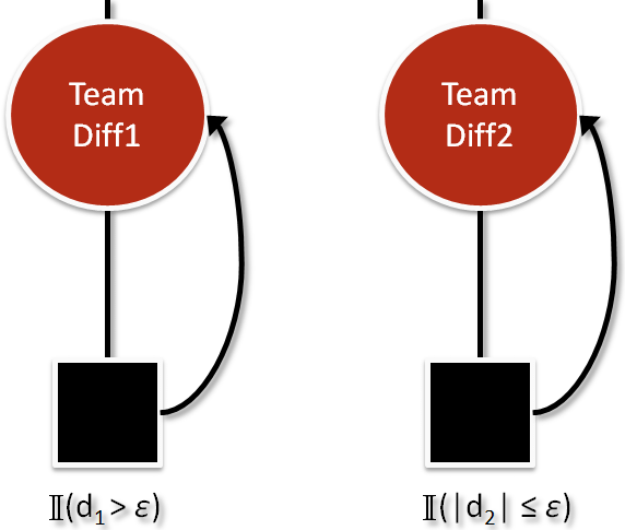
The comparison depends on whether the pairwise difference was considered a “win” or a “draw.” Obviously, this depends on the rules of the game. It’s important to realize that TrueSkill only cares about these two types of results. TrueSkill doesn’t care if you won by a little or a lot, the only thing that matters is if you won. Additionally, in TrueSkill we imagine that there is a buffer of space called a “draw margin” where performances are equivalent. For example, in Olympic swimming, two swimmers can “draw” because their times are equivalent to 0.01 seconds even though the times differ by several thousandths of a second. In this case, the “draw margin” is relatively small around 0.005 seconds. Draws are very common in chess at the grandmaster level, so the draw margin would be much greater there.
The output of the comparison factor directly relates to how much your skill’s mean and standard deviation will change.
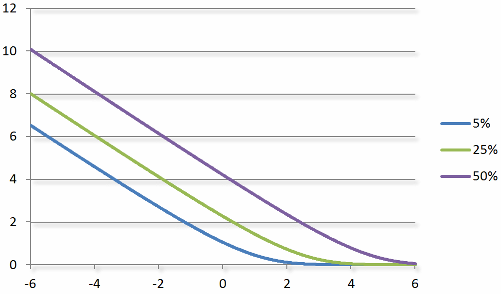
The exact math involved in this factor is complicated, but the core idea is simple:
- Expected outcomes cause small updates because the algorithm already had a good guess of your skill. - Unexpected outcomes (upsets) cause larger updates to make the algorithm more likely to predict the outcome in the future.
The accompanying math paper goes into detail, but conceptually you can think of the performance difference as a number on the bottom (x-axis) of a graph. It represents the difference between the expected winner and the expected loser. A large negative number indicates a big upset (e.g. an underdog won) and a large positive number means the expected person won. The exact update of your skill’s mean will depend on the probability of a draw, but you can get a feel for it by looking at this graph:
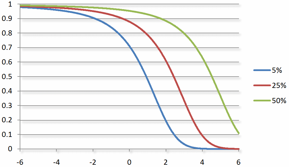
Similarly, the update to a skill’s standard deviation (i.e. uncertainty) depends on how expected the outcome was. An expected outcome shrinks the uncertainty by a small amount (e.g. we already knew it was going to happen). Likewise, an unexpected outcome shrinks the standard deviation more because it was new information that we didn’t already have:
One problem with this comparison factor is that we use some fancy math that just makes an approximation (a good approximation, but still an approximation). We’ll refine the approximation in the next step.
The Inner Schedule: Iterate, Iterate, Iterate!
We can make a better approximation of the team difference factors by passing around the messages that keep getting updated in the following loop:
After a few iterations of this loop, the changes will be less dramatic and we’ll arrive at stable values for each marginal.
Enough Already! Give Me My New Rating!
Once the inner schedule has stabilized the values at the bottom of the factor graph, we can reverse the direction of each factor and propagate messages back up the graph. These reverse messages are represented by black arrows in the graph of each factor. Each player’s new skill rating will be the value of player’s skill marginal variable once messages have reached the top of the factor graph.
By default, we give everyone a “full” skill update which is the result of the above procedure. However, there are times when a game title might want to not make the match outcome count much because of less optimal playing conditions (e.g. there was a lot of network lag during the game). Games can do this with a “partial update” that is just a way to apply only a fraction of the full update. Game titles specify this via the X_PROPERTY_PLAYER_SKILL_UPDATE_WEIGHTING_FACTOR variable. I implemented this feature in the accompanying source code and describe it in the math paper.
Results
There are some more details left, but we’ll stop for now. The accompanying math paper and source code fill in most of the missing pieces. One of the best ways to learn the details is to implement TrueSkill yourself. Feel free to create a port of the accompanying project in your favorite language and share it with the world. Writing your own implementation will help solidify all the concepts presented here.
The most rewarding part of implementing the TrueSkill algorithm is to see it work well in practice. My coworkers have commented on how it’s almost “eerily” accurate at computing the right skill for everyone relatively quickly. After several months of playing foosball, the top of the leaderboard (sorted by TrueSkill: the mean minus 3 standard deviations) was very stable. Recently, a very good player started playing and is now the #2 player. Here’s a graph of the most recent changes in TrueSkill for the top 5 (of around 40) foosball players:
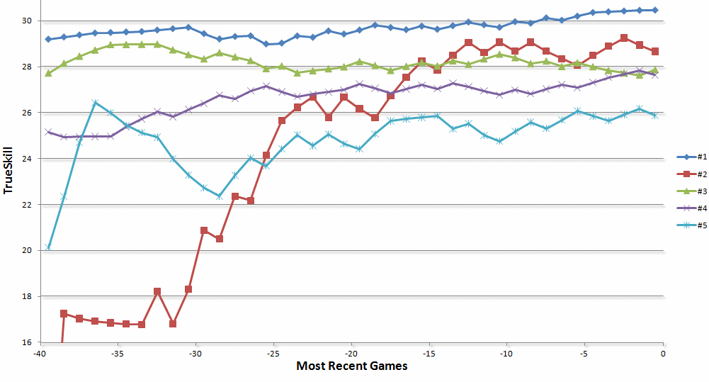
(Note: Look how quickly the system detected how good this new #2 player is even though his win ratio is right at 50%)
Another interesting aspect of implementing TrueSkill is that it has raised an awareness of ratings among players. People that otherwise wouldn’t have played together now occasionally play each other because they know they’re similarly matched and will have a good game. One advantage of TrueSkill is that it’s not that big of a deal to lose to a much better player, so it’s still ok to have unbalanced games. In addition, having ratings has been a good way to judge if you’re improving in ability with a new shot technique in foosball or learning more chess theory.
Fun Things from Here
The obvious direction to go from here is to add more games to the system and see if TrueSkill handles them equally well. Given that TrueSkill is the default ranking system on Xbox live, this will probably work out well. Another direction is to see if there’s a big difference in TrueSkill based on position in a team (e.g. midfield vs. goalie in foosball). Given TrueSkill’s sound statistics based on ranking and matchmaking, you might even have some success in using it to decide between to several options. You could have each option be a “player” and decide each “match” based on your personal whims of the day. If nothing else, this would be an interesting way to pick your next vacation spot or even your child’s name.
If you broaden the scope of your search to using the ideas that we’ve learned along the way, there’s a lot more applications. Microsoft’s AdPredictor (i.e. the part that delivers relevant ads on Bing) was created by the TrueSkill team and uses similar math, but is a different application.
As for me, it was rewarding to work with an algorithm that has fun social applications as well as picking up machine learning tidbits along the way. It’s too bad all of that didn’t help me hit the top of any of the leaderboards.
Oh well, it’s been a fun journey. I’d love to hear if you dived into the algorithm after reading this and would especially appreciate any updates to my code or other language forks.
Links:
- The Math Behind TrueSkill - A math-filled paper that fills in some of the details left out of this post. - Moserware.Skills Project on GitHub - My full implementation of Elo and TrueSkill in C#. Please feel free to create your own language forks. - Microsoft’s online TrueSkill Calculators - Allows you to play with the algorithm without having to download anything. My implementation matches the results of these calculators.
Special thanks to Ralf Herbrich, Tom Minka, and Thore Graepel on the TrueSkill team at Microsoft Research Cambridge for their help in answering many of my detailed questions about their fascinating algorithm.